Longitudinal Analysis #

Author - John L. Korey
Department of Political Science
California State Polytechnic University, Pomona
e-mail: JLKorey@gmail.com

© The Author, 2016. Last Modified December 5, 2016.[1]

#Winner of a 2019 MERLOT Classic Award in Sociology

These exercises introduce you to several ways of analyzing data over time. Although many different sorts of data may be subject to longitudinal analysis, we'll be focusing on surveys of public opinion. Data for the exercises consist of three subsets drawn from two well-known national surveys, the General Social Survey (GSS) and the American National Election Study (ANES). Data analysis is done using a statistical package called SPSS. The data are freely available for your use. Use of SPSS does require that you have a license. There is a good chance that your college or university has a site license for SPSS. If not, you can rent a student license. Except for the line graphs, you can also do the exercises using PSPP, a freely available statistical analysis package with a look and feel very similar to SPSS.

PRELIMINARIES

Those needing an introduction to, or refresher on, SPSS should consult SPSS for Windows Version 23.0: A Basic Tutorial (Edward Nelson, Editor). In the box above, you'll find links to the full Tutorial as well as to specific chapters (and, in some cases, specific pages ("bookmarks") used in these exercises. For other sites providing instruction on SPSS, see the SPSS section of the Social Science Research and Instructional Council’s “Links to Other Instructional Sites”.

We’ll be analyzing three data subsets created for these exercises, two drawn from the General Social Survey (GSS) and one from the American National Election Studies (ANES). In each case, a codebook describing the variables included in the subset is also included in PDF format.

• The first of these is a subset (data: gsscum.sav; codebook: gsscum.pdf) of the GSS 1972-2014 Cumulative File, which includes all respondents surveyed from the first GSS through the most recently available at this writing.[2]
• The second is a subset (data: gsspanel.sav; codebook: gsspanel.pdf) of a three wave GSS panel study in which respondents to the 2010 study were re-interviewed in 2012 and 2014.
• The third is a subset (data: anespanel.sav; codebook: anespanel.pdf) of a five wave panel study in which respondents to the 2000 ANES pre-election study were re-interviewed after the election, again both before and after the 2002 election, and after the 2004 election. 

Most of the variables included in the subsets are taken directly from the full studies[3]. In a few instances, we have modified variables or created new ones using the “Recode” and “Compute” features of SPSS. Both datasets and codebooks can be downloaded using the links at the beginning of these exercises[4].

INTRODUCTION

Most sample surveys involve cross-sectional analysis.   That is, they provide us with a snapshot sample of a population at a single point in time. Time, however, is itself one of the most important variables in politics. The study of change over time is called longitudinal analysis.  Here we will focus on the study of change over time in public opinion and behavior, as measured through sample surveys.  Longitudinal analysis of survey data can be subdivided into three types: trend analysis, cohort analysis, and panel studies. We will cover each of these in turn.

TREND ANALYSIS

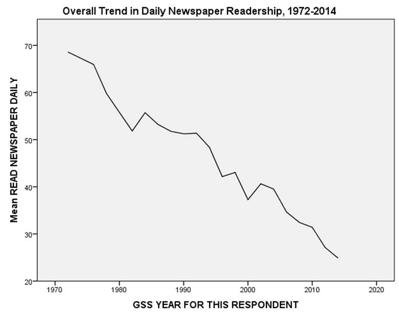
The simplest type of longitudinal analysis of survey data is called trend analysis, which examines overall change over time.  A good example of change over time can be seen Figure 1, showing the dramatic decline in newspaper readership that occurred in the United States between 1972 and 2014. The decline in readership and revenue of “legacy” (a.k.a. “dead tree”) media has, not surprisingly, produced considerable hand-wringing among many journalists[5].

Figure 1

You can produce this figure with a simple LINE CHART in SPSS, using data from the GSS Cumulative File Subset (gsscum.sav) and explanations of the data from the codebook (gsscum_codebook.pdf). You will need to WEIGHT CASES by weight to correct for known discrepancies between the characteristics of the sample and the population from which it was drawn. Choose year for the horizontal (x) axis, and news for the vertical (y) axis. If you select Mean as the statistic represented by the line, it can be interpreted as the percentage of respondents reporting that they read a newspaper on a daily basis. (We’ll explain this more fully below.)

In the first year surveyed, about two-thirds of all respondents reported reading a newspaper on a daily basis.  Thereafter, regular newspaper readership more or less continuously declined until, by 2014, only about a quarter of respondents were daily readers.  (Note: look for overall trends, and do not get too caught up in short-term fluctuations.  The slight rise in newspaper readership in 2002, for example, might have indicated a reversal in the downward trend, but seems to have been due to short term forces or perhaps merely sampling error.)

Trend analysis has some significant limitations.  While it can reveal change, it gives us little insight as to how or why the changes have taken place. We might, for example, suspect that attitudes and behaviors are related to similarities and differences between generations. First, individuals in every generation may change as they move through the life cycle; simply put, as people get older, their perspectives change, for better and/or worse. Second, people may change because of new circumstances.  Technological developments, or a major crisis such as a war or depression, may result in similar changes that impact all age groups in a similar way.  Finally, change may be the result of cohort replacement.  Different generations are shaped by different experiences.  Events that occur as people are coming of age are likely to have a big impact on their outlooks, and this impact may prove lasting, continuing to influence them for the rest of their lives.  Even if no individual ever changed after reaching adulthood, overall change would occur as one generation dies out and another generation, having gone through different formative experiences, comes on the scene.

COHORT ANALYSIS

One way to sort some of this out is through cohort analysis.   There are many different types of cohorts. For example, people surveyed at different times who had the same level of education might be considered an educational cohort. We could see whether the overall trend shown in Figure 1 has differed from one educational cohort (for example, college graduates) to another (for example, those with less than a high school diploma).

We’re going to focus here on age categories. People born during the same time period are considered to form an age cohort.  For example, respondents in their 20s in a 1980 survey belong to the same age cohort as respondents in their 50s in a 2010 survey.  By comparing respondents from the same age cohort surveyed at different times, we can measure change over time in the attitudes and behavior within the cohort. 

To illustrate this, we will again use the General Social Survey (GSS) cumulative file subset. Respondents have been divided into the following:

The GI Generation (born 1927 or earlier — the earliest year of birth reported by respondents to any of the General Social Surveys is 1883)

Members of this cohort were at least 18 years old by the end of 1945, the year World War II ended.  This generation lived through the Great Depression of the 1930s, the New Deal, and the Second World War.  All Presidents of the United States from Truman through the first President Bush came from this cohort.

The Silent Generation (born 1928.-1945)

This generation came of voting age after World War II, but before most of the political turbulence of the late 1960s. The youngest members of the cohort turned 18 the year John Kennedy was assassinated. Because its members reached adulthood in relatively placid times and because it is a relatively small cohort, this group has sometimes been labeled the “silent” generation. At this writing (2016), it has yet to produce a president, though four members, Walter Mondale (born 1928), Michael Dukakis (1933), John McCain (1936), and John Kerry (1943), received major party presidential nominations.

The Baby Boomers (born 1946-1964)

During the Depression and the Second World War, the United States experienced a low birth rate. This changed dramatically after the war ended. The birth rate remained high until the mid-1960s. As a result, the generation born during these years would come to constitute an unusually large portion of the overall population and, as a result, has drawn an unusual amount of attention. It was this generation that was on college campuses in the late sixties at a time of great turmoil over the War in Vietnam, civil rights, and a variety of other issues. Today, the older members of this cohort are retiring and, as they do, an enormous strain is being placed on the federal budget as entitlements burgeon in the Social Security and Medicare programs. Bill Clinton, George W. Bush, and Donald Trump (all born in 1946), and Barack Obama (1961) are “boomers.” 

Generation X (born 1965-1981)

The “baby boom” was followed by the “baby bust” as birth rates plummeted. Called “Gen X” because, by some reckonings, this is the tenth generation of Americans since independence (hence the Roman numeral “X”), older members of this generation came of voting age during the administrations of Ronald Reagan and the first President Bush. Younger members attained adulthood during the Clinton Administration. Members of this cohort are eligible to become president, but none have done so as yet.

The Millennium Generation (1982-1999).

Members of this cohort are called Millennials because they were born before 2000, and came of voting age (and are still doing so) during or after that year. Like the Boomers, Millennials are an unusually large cohort, and thus likely to have an especially big impact on American politics. The cohort’s oldest members, however, will not turn 35, and thus become eligible for the presidency, until the 2020 election. 

Figure 2

For background purposes, Figure 2 graphs the changing composition of the General Social Survey from 1972 through 2014.  The same information is presented in tabular form below the graph, with numbers representing percentages of the total sample.  The GI Generation provides half of the respondents to the 1972 survey, declining thereafter to only one percent of all respondents in 2014.  The Silent Generation is a relatively small cohort, never reaching more than about a third of all respondents, and reduced to about an eighth in 2014.  The Baby Boomers reached their peak of representation in 1984 (45 percent), and still constituted about a third of the total in 2014.  The leading edge of Generation X entered the sample in 1984, and reached 36 percent in 2002.  By 2014, Millennials constituted a fourth of the sample.

As noted earlier, an overall trend, or lack thereof, may be explained in several ways.  First may be a new development that affects all cohorts equally, either suddenly or gradually.  If this is the case, trend lines should be similar for each cohort.  Second, there may be life cycle factors at work.  If, for example, people tend to become more conservative as they get older, an analysis of ideology would show each cohort starting out liberal and then becoming more conservative over time.  The trend line for each cohort would be in the same direction, but the change for each generation would lag that of the one preceding it.  Third, a trend may occur as a result of generational replacement — there may be little within-cohort change over time, but an older generation may pass from the scene and be replaced by a new generation with different attitudes or behaviors.  Of course, two or more of these factors may combine to produce the overall pattern.

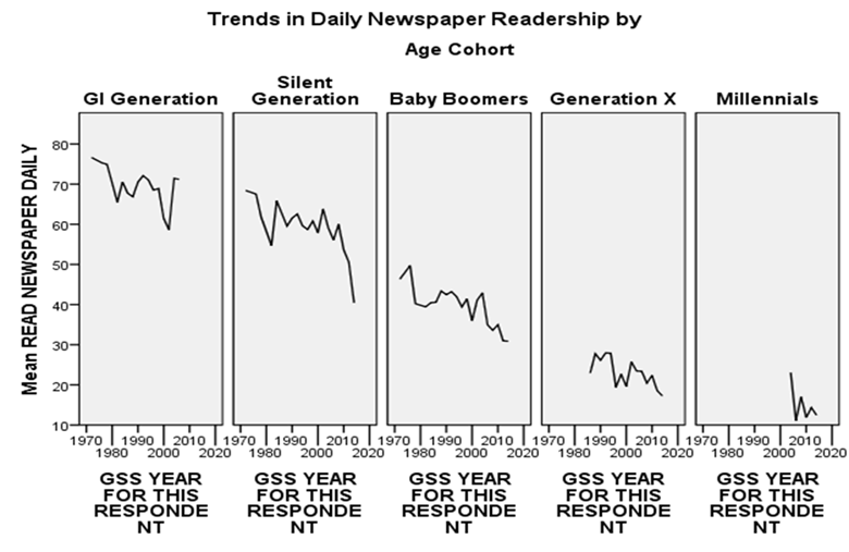
Figure 3

To see how cohort analysis can be applied to study change over time, consider Figure 3, which breaks trends in daily newspaper readership down by age cohort. You can produce this figure with a multiple LINE CHART in SPSS, using cohort as the panel variable.

There does seem to be some tendency, especially among the Boomers, for newspaper readership to decline over time within cohorts. The most dramatic differences, however, are between cohorts.  Note that the line for the Boomers is entirely above that of Generation X and almost entirely below that of the Silent Generation. Among Millennials, daily newspaper readership has practically vanished. In other words, the overall trend away from daily newspaper reading is due mainly to generational replacement.  Habits established early in life seem to persist, but older readers are dying out.  Each generation is less devoted to the daily newspaper than its predecessor. For a long time now, newer cohorts have turned to newer media: first television, then online media.

Now let’s look at how responses to some other items in the GSS have changed over time. Repeat the above analyses, but instead of news, try other variables in the subset that you think might be interesting. To facilitate analysis, all attitudinal and behavioral variables in this subset have been recoded to form dichotomies, with valid values of 0 and 100.  Variables were recoded to divide respondents into groups that are as nearly equal in size as possible. The mean score of the variable on the vertical axes of the line charts can be interpreted as the percent of respondents choosing one side of the dichotomy. Be sure to select mean as the statistic represented by the lines.

Try the same sort of analysis using cohorts not based on age. Instead of using cohort as your panel variable, use any of the demographic variables found in the codebook from degree though attend. To keep the number of cohort categories manageable, and to avoid categories with too few cases to be reliable, you may need to RECODE some of these variables.

PANEL STUDIES

While cohort analysis allows us to extract more information from our data than an overall trend analysis, it still suffers from some serious limitations.  While people who were surveyed while in their twenties in 1974 were drawn from the same age cohort as people in their sixties interviewed in 2014, they are not the same people.  Both surveys are subject to random sampling error, and this may produce some of the changes we observe. 

For this reason, the “gold standard” for longitudinal analysis of survey data is the panel study. In a panel, the same people are interviewed at two or more points in time. Since the sample is the same, any changes we observe are not a result of random sampling error.

Panel studies, however, have problems of their own. For one thing, they are generally very expensive, since great effort has to be expended to keep track of respondents.   For another, despite our best efforts, researchers will not be successful in all of their attempts to recontact respondents, especially if the study is conducted over a long period of time. This dropoff in respondents is called “attrition.”   Those who drop out of the panel (by moving, dying, refusing to continue, etc.) might have differed in their attitudes and behaviors from those who remain. Finally, there is the problem of reactivity. When respondents are interviewed, their interest in politics may be piqued. If they know that they will be interviewed again, they may even tend to study up on politics so as not to appear ignorant. By the end of the study, what started off as a representative sample may have become something of an elite group.

With cohort analysis, we examined how whole groups (in this case, generations) of people change over time. With panel studies, we look at change in a different way; because these studies interview the same people at different times, we can focus on what happens at the individual level as well as at the group (or aggregate) level.

To illustrate the use of panel studies, we’ll look first at one conducted in three waves (2010, 2012, and 2014) by NORC’s General Social Survey. We’ll use this study to examine two important concepts in social research: cognitive dissonance and reactivity.

Cognitive Dissonance[6]

Cognitive dissonance refers to the stress people may encounter when holding two paradoxical views. This may result in psychological pressure to reduce the dissonance by changing one’s views to bring them closer into alignment. We’ll focus specifically on the dissonance that might result from having a party identification that’s a poor fit for one’s political ideology, as would be the case for liberal Republicans or conservative Democrats. (Such people are sometimes referred to as “caught behind enemy lines.”) The theory of cognitive dissonance would lead us to predict that such people would tend to rethink their party loyalties, their views on issues, or both[7].

Open the General Social Survey 2010-2014 Panel Survey Subset Codebook (gsspanel_codebook.pdf). For the subset, we’ve created some additional variables for this exercise. (We'll be "crosstabulating" these variables. For a brief introduction to crosstabulation, follow this link.

dissonance.  The GSS measures party identification on a seven point scale from Strong Democrat to Strong Republican, and measures political ideology on another seven point scale from extremely liberal to extremely conservative. Respondents are self-identified on both scales. Our dissonance variable measures the difference if any between these two scores in 2010 on a three point scale as follows

1. High Dissonance (more conservative than Republican): further toward the conservative end of the ideology scale than toward the Republican end of the party ID scale. Those in this category are at least two points further to the “right” on ideology than on party ID.
2. No or Low Dissonance. Those in this category have scores on the two scales that differ by no more than one point.
3. High Dissonance (more liberal than Democratic): further toward the liberal end of the ideology scale than toward the Democratic end of the party ID scale. Those in this category are at least two points further to the “left” on ideology scale than on party ID.

ptychange. This variable measures the change, if any, in a respondent’s party identification between 2010 and 2014. Using the same seven point scale described above, this variable has a range of -6 (a move from strong Republican to strong Democrat) to 6 (the opposite).

viewchange. This variable measures the change, if any, in a respondent’s political ideology between 2010 and 2014. Using the same seven point scale described above, this variable has a range of -6 (a move from extremely conservative to extremely liberal) to 6 (the opposite).

We’ve chosen the 2010 and 2014 surveys because both party ID and political ideology are relatively stable, and so we wanted to allow sufficient time to pass for respondents to change their minds.

Cognitive dissonance theory would lead us to predict that those with:

Hypothesis I

A.  high dissonance (more conservative than Republican) in 2010 will tend to reduce that dissonance by shifting their party IDs in the direction of the Republican Party between 2010 and 2014, and.

B.  low or no dissonance will tend to show little or no movement in party ID between 2010 and 2014, and.

C.  high dissonance (more liberal than Democratic) will tend to reduce that dissonance by shifting their party IDs in the direction of the Democratic Party between 2010 and 2014.

Hypothesis II

Similarly, cognitive dissonance theory would also lead us to predict that those with:

A.   high dissonance (more conservative than Republican) in 2010 will tend to reduce that dissonance by shifting their political views in the direction of greater liberalism between 2010 and 2014, and

B.   low or no dissonance will tend to show little or no movement in their political ideology between 2010 and 2014, and

C.  high dissonance (more liberal than Democratic) will tend to reduce that dissonance by shifting their political ideology in the direction of greater conservatism between 2010 and 2014.

Start SPSS, and open the GSS 2010-2014 subset (gsspanel.sav). Test the above hypotheses with CROSSTABS of ptychange and viewchange (dependent variables) with dissonance (independent variable). WEIGHT CASES by wtpannr123. What measures of significance and association will you use?[8] Do your findings support one or both hypotheses? Explain.

Reactivity[9]

Reactivity refers to the fact that, in the very act of measuring something, we may alter the results. In survey research, this may occur when a “loaded” question biases the answers obtained. An extreme (and highly unethical) example of this is a “push poll” in which this is done deliberately, not in order to obtain information, but in order to influence voters through disinformation. Example: “If you knew that candidate X had embezzled funds, would this make you more likely to vote for him/her in the upcoming election for city treasurer, less likely, or would it make no difference?” (P.S., there is, in fact, no evidence that candidate X has ever been an embezzler.)

Sometimes, reactivity can occur in more subtle ways. In the surveys included in the 2010-2014 panel, the GSS asked respondents whether they agreed or disagreed that “a preschool child is likely to suffer if his or her mother works.” We might hypothesize that the answer given to this question will be influenced by various characteristics (e.g., gender) of the respondent[10]. Respondents might hesitate to tell a female interviewer, who obviously works outside the home and who might have preschool children, that they believe her work would be harmful to them. Since about 80 percent of the interviewers employed by the GSS are women this could, if true, skew the overall results in the direction of overestimating disagreement with the question.

We’ll focus on the 2010 and 2012 surveys. We’ve chosen the 2012 survey rather than the one from 2014 because it suffers somewhat less from attrition, and therefore provides more, and possibly better, data. In addition, the percentage of female interviewers was even higher in 2014 than in the other two surveys.

Open the General Social Survey 2010-2014 Panel Survey Subset Codebook (gsspanel_codebook.pdf). To test for reactivity, we’ve created two new variables:

 intchange, that breaks respondents down into those interviewed by a:

1. person of the same gender in both 2010 and 2012,
2. man in in 2010 and by a woman in 2012, and
3. woman in 2010 and by a man in 2012;

 anschange, that breaks respondents down into those who:

1. answered the question the same way in both 2010 and 2012,
2. agreed in 2010 but disagreed in 2012, and
3. disagreed in 2012 but agreed in 2010.

Start SPSS, and open the GSS 2010-2014 subset (gsspanel.sav). WEIGHT CASES by wtpannr12.  (This differs from the weight variable used above in that it doesn’t include an adjustment for 2014. Note that, since this weight variable doesn’t apply to those who weren’t surveyed in 2014, you may get warning messages with your output. Ignore them.)

CROSSTAB anschange by intchange. Test for statistical significance and association. To the extent that you see evidence of reactivity, these statistics should cause you to view such evidence very skeptically. Why?

For our last two exercises, we’ll use a subset of the 2000-2004 panel study conducted as part of the American National Election Study.

Regression Toward the Mean vs. Polarization

Let’s suppose (though it may not be true in every case), that last term you not only got straight “A” grades, but that you got perfect scores on every quiz, test, and paper. You must be a pretty good student, and should do well this term as well. Odds are, though, that you won’t do quite as well this time as last. To perform as well as you did, you likely had everything going for you: a “perfect storm” of your own hard work and of circumstances beyond your control. This time around, you might (not saying you will) slack off a bit, be taking an especially tough course, or come down with a bad cold right before an important exam. If this happens, and your grades aren’t quite as exemplary as they were, blame it on “regression toward the mean.”[11]

The ANES panel study measures party identification along a seven point scale ranging from Strong Democrat through Independent to Strong Republican.[12] We have recoded this variable for the 2000 and 2004 pre-election surveys into four categories: strong identifiers, weak identifiers, leaners, and pure independents, and named the resulting variables ptystr00 and ptystr04. Regression toward the mean would suggest that respondents who change party identification over time will have a tendency, all else being equal, to move from stronger to weaker identification or toward pure independence.[13]

All else, however, is probably not equal. If it were, all voters would ultimately end up as pure independents. In fact, a great deal has been written pointing to a growing partisan polarization in America, a trend that has been going on since the 1970s. This would suggest that voters have been moving, not toward the center, but toward stronger party identification. We can test both of these competing hypotheses using the recoded party identification scale. We’ll focus on the presidential election years of 2000 and 2004.

Start SPSS. Open the ANES 2000-2002-2004 Panel Study Subset (anespanel.sav) and the ANES 2000--2002-2004 Panel Study Subset Codebook (anespanel_codebook.pdf). WEIGHT CASES by wt04. Crosstab ptystr04 (as dependent variable) by ptystr00 (as independent variable). Do more respondents move toward weaker (or no) party ID, or toward stronger, or do the two movements more or less cancel out?

The Nader Effect

The 2000 presidential race between Republican George W. Bush and Democrat Al Gore came down to Florida, with its bloc of 25 Electoral College votes. The popular vote there was a virtual tie, with the outcome dependent on how disputes over some ballots would be resolved. In the end, George W. Bush was declared the winner by 537 votes out of almost 6 million cast. Green Party candidate Ralph Nader garnered 103,759 votes. Since Nader ran to the left of Gore, most observers agreed that, had Nader not been in the race, Gore would have won Florida by a close but decisive margin and, with it, the presidency. Some Democrats blamed Nader (along with some guy named “Chad”[14]) for their defeat.

To what extent did Nader’s role in the 2000 election influence negatively impact his popularity with Democrats in the days and years that followed? In both the pre- and post-election 2000 surveys, in the 2002 pre-election survey, and in the 2004 post-election survey, the ANES included “feeling thermometers,” asking respondents to rate Nader (among other individuals and groups) on a scale of 0 to 100, with 100 indicating very “warm” (i.e., favorable) feelings, 50 indicating neutral feelings, and 0 indicated very “cold” feelings. In the 2000 pre-election survey, how did Democrats in the panel compare with independents and Republicans in their feelings toward Nader? Did this change in the days immediately following the election (i.e., in the post-election survey)? Were there further changes in 2002 and in 2004?

By using the 2000 pre-election wave as a baseline, we can see that, prior to that year’s election, Republicans clearly viewed Nader less favorably (mean rating, including Republican “leaners”:  42.48) than either independents (mean rating: 55.41) or Democrats (mean rating: 55.04).

We’ve created new variables to measure subsequent change in feelings about Nader: 1) rnchng00, the score a respondent gave Nader in the 2000 post-election survey minus his score in that year’s pre-election survey, 2) rnchng02, his score in the 2002 post-election survey minus his 2000 pre-election score, and 3) rnchng04, his score in the 2004 post-election survey minus his 2000 pre-election score.  In each case, a positive score indicates that the respondent liked Nader better after the later survey than on his baseline score prior to the 2000 election.

Start SPSS.  Open the ANES 2000-2002-2004 Panel Study Subset (anespanel.sav) and the ANES 2000--2002-2004 Panel Study Subset Codebook (anespanel_codebook.pdf). WEIGHT CASES by wt04. Do a COMPARE MEANS test with the three measures of change in Nader’s thermometer scores as dependent variables, and ptyid300 as the independent variable. (Note: three point party ID scores have been recoded to combine independents and those identifying with a minro party.) Explain your results.

KEY CONCEPTS

age cohort
cohort analysis
cross sectional analysis
cohort replacement
cognitive dissonance
longitudinal analysis
panel study
reactivity
trend analysis

FOR FURTHER STUDY

Nelson, Elizabeth N., and Edward E. Nelson, “Research Design and Methods of Analysis for Change Over Time,” California Opinions on Women's Issues — 1985-1995 ssric.org/trd/modules/cowi/chapter6.  August 15, 1998.  Accessed August 22, 2016.

Palmquist, Ruth A., “Survey Methods,” https://www.ischool.utexas.edu/~palmquis/courses/survey.html.  Accessed August 22, 2016.

Ruspini, Elisabetta, “Longitudinal Research in the Social Sciences,” Social Research Update. http://sru.soc.surrey.ac.uk/SRU28.html.  Spring, 2000.  Accessed August 22, 2016.  

[1] Licensed under a  Creative Commons Attribution-Noncommercial-Share Alike 3.0 Unported License. An earlier version of these exercises appeared as part of Introduction to Research Methods in Political Science: The POWERMUTT Project.

[2] Starting in 1972, the GSS has been conducted in every even numbered year except for 1992.  Prior to 1994, it was also conducted in odd numbered years. For consistency, and to facilitate presentation, all surveys from odd numbered years have been combined with the survey from the following year and coded as such (e.g., the 1973 survey is treated as part of the 1974 survey). This includes the 1991 survey, which was coded as 1992, even though no survey was conducted in 1992. In addition, a cohort has been excluded in any year for which it was represented by fewer than 100 respondents.

[3] For the ANES subset, original variable names have been replaced with ones that are more intuitive. For example, m000092 has been renamed region. 

[4] You can also download the full studies from which the subsets are taken by going to http://gss.norc.org/Get-The-Data (GSS 1972-2014 Cross-Sectional Cumulative Data; GSS Panel 2010-Sample Wave 3) and http://www.electionstudies.org/studypages/download/datacenter_all_NoData.php  (ANES 2000-2004 Merged File: free registration required).

[5] Jordan Weissmann, “The Decline of Newspapers Hits a Stunning Milestone,” Slate http://www.slate.com/blogs/moneybox/2014/04/28/decline_of_newspapers_hits_a_milestone_print_revenue_is_lowest_since_1950.html. April 28 2014. Accessed September 1, 2016.

[6] Saul McLeod, “Cognitive Dissonance,” Simply Psychology http://www.simplypsychology.org/cognitive-dissonance.html. 2014. Accessed September 10, 2016.

[7] A third alternative would be to “leave the field” by losing interest in politics, which would not necessarily reduce the level of cognitive dissonance, but would reduce its “salience,” or perceived importance. Unfortunately, a variable that would provide a good test of this (polint) was not included in the 2010 or 2012 surveys.

[8] See John L. Korey, Introduction to Research Methods in Political Science http://www.cpp.edu/~jlkorey/POWERMUTT/Topics/contingency_tables.html. April 28, 2013. Accessed September 10, 2016.

[9] David P. French and Stephen Sutton, “Methods: Does Measuring People Change Them?” The Psychologist,vol. 24 . https://thepsychologist.bps.org.uk/volume-24/edition-4/methods-does-measuring-people-change-them. April 2011. Accessed September 12, 2016.

[10] Men and women did in fact answer this question somewhat differently. Though majorities of both men and women disagreed with the statement, men were between 11 and 13 percentage points more likely than were women to agree.

[11] If you’ve taken a course in statistics, you’ve probably been introduced to “regression analysis,” also called “ordinary least squares” (OLS).  It is called regression analysis because Francis Galton (1822-1911), a pioneer in the application of OLS to the behavioral sciences, used it to study “regression toward the mean.” See A. Abebe, J. Daniels, J. W. McKean , and J. A. Kapenga, “How Regression Got Its Name,”  Statistics and Data Analysis. http://www.stat.wmich.edu/s160/book/node70.html.  January 1, 2001.  Accessed September 1, 2016.

[12] The scale is constructed by ANES from two questions asked of respondents. The first is: "Generally speaking, do you usually think of yourself as a Republican, a Democrat, an Independent, or what?" If respondents answer that they are Republican or Democrat, they are then asked: "Would you call yourself a strong Republican/Democrat or a not very strong Republican/Democrat?” If respondents answer the first question by saying that they are independent, something other, or have no preference, they are asked: "Do you think of yourself as closer to the Republican or Democratic party?"

[13] Pure independents don’t precisely represent the mean, but in the base year of 2000 they came pretty close to doing so. The ANES scale ranges from 0 (Strong Democrat) to 6 (Strong Republican), with a mean in 2000 of 2.96 (in other words, just slightly favoring the Democrats).

[14] In 2000, local jurisdictions in Florida used a variety of different ballot formats, including cards with devices that voters used to punch holes in their cards next to their choices for each office. The rectangle thus punched out is called a “chad.” Sometimes, the effort would be only partly successful, leaving a “hanging” chad with one or more corners not removed. Election officials then had to decide, with no clear standards in state law to guide them, whether the chad had been removed sufficiently to indicate a clear preference.