Author: Ed Nelson
Department of Sociology M/S SS97
California State University, Fresno
Fresno, CA 93740
Email: ednelson@csufresno.edu
Note to the Instructor: This exercise uses the 2014 General Social Survey (GSS) and SDA to explore measures of association. SDA (Survey Documentation and Analysis) is an online statistical package written by the Survey Methods Program at UC Berkeley and is available without cost wherever one has an internet connection. The 2014 Cumulative Data File (1972 to 2014) is also available without cost by clicking here. For this exercise we will only be using the 2014 General Social Survey. A weight variable is automatically applied to the data set so it better represents the population from which the sample was selected. You have permission to use this exercise and to revise it to fit your needs. Please send a copy of any revision to the author. Included with this exercise (as separate files) are more detailed notes to the instructors and the exercise itself. Please contact the author for additional information.
I’m attaching the following files.
- Extended notes for instructors (MS Word; .docx format).
- This page (MS Word; .docx format).
Goals of Exercise
The goal of this exercise is to introduce measures of association. The exercise also gives you practice in using CROSSTABS in SDA.
Part I—Relationships between Variables
We’re going to use the General Social Survey (GSS) for this exercise. The GSS is a national probability sample of adults in the United States conducted by the National Opinion Research Center (NORC). The GSS started in 1972 and has been an annual or biannual survey ever since. For this exercise we’re going to use the 2014 GSS. To access the GSS cumulative data file in SDA format click here. The cumulative data file contains all the data from each GSS survey conducted from 1972 through 2014. We want to use only the data that was collected in 2014. To select out the 2014 data, enter year(2014) in the Selection Filter(s) box. Your screen should look like Figure 11_1. This tells SDA to select out the 2014 data from the cumulative file.
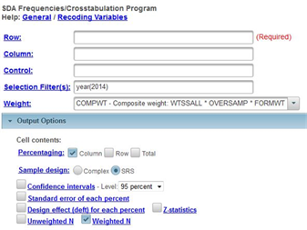
Figure 11-1
Notice that a weight variable has already been entered in the WEIGHT box. This will weight the data so the sample better represents the population from which the sample was selected.
There’s one other thing that it’s important to do. Click on the arrow next to OUTPUT OPTIONS and look at the line that says SAMPLE DESIGN. On your screen COMPLEX will be selected. Click on the circle next to SRS to select it.
The GSS is an example of a social survey. The investigators selected a sample from the population of all adults in the United States. This particular survey was conducted in 2014 and is a relatively large sample of approximately 2,500 adults. In a survey we ask respondents questions and use their answers as data for our analysis. The answers to these questions are used as measures of various concepts. In the language of survey research these measures are typically referred to as variables. Often we want to describe respondents in terms of social characteristics such as marital status, education, and age. These are all variables in the GSS.
In a previous exercise (STAT9S_SDA) we used crosstabulation and percents to describe the relationship between pairs of variables in the sample. In exercise STAT10S_SDA we went beyond simple description. We used the sample data to make inferences about the population from which the sample was selected. Chi Square was used to test hypotheses about the population. Chi Square is the appropriate test when your variables are nominal or ordinal (see STAT1S_SDA).
Chi Square is a test of the null hypothesis that two variables are unrelated to each other. Another way to put this is that the two variables are independent of each other. If we can reject the null hypothesis then we have support for our research hypothesis that the two variables are related to each other. But showing that two variables are related is not the same thing as determining the strength of the relationship. The strength of a relationship is actually a continuum from very weak to very strong. To measure the strength of a relationship we need to select and compute a measure of association. In this exercise we’re going to focus on nominal and ordinal variables. In exercises STAT13.1S_SDA and STAT13.2S_SDA we’ll talk about measures for interval and ratio variables.
Part II – What is a Measure of Association?
Before we discuss measures of association, we need to talk about independent and dependent variables. The dependent variable is whatever you are trying to explain. For example, let’s say we want to find out why some people think that abortion should be legal and others think it should be illegal. The independent variable is some variable that you think might help you answer this question. Perhaps we decide to use sex as our independent variable.
A measure of association is a numerical value that tells us how strongly related two variables are. There are several characteristics of a good measure of association.
- They range from a value of 0 (i.e., no relationship) to 1 (i.e., the strongest possible relationship).
- For variables that have an underlying order from low to high they can be positive or negative. A positive value indicates that as one variable increases, the other variable also increases. A negative value indicates that as one variable increases, the other variable decreases.[1]
- Some measures specify which variable is dependent and which is independent. The independent variable is some variable that you think might help explain the variation in the dependent variable. For example, if your two variables were education and voting you might choose education as the independent variable and voting as your dependent variable because you think that education will help you explain why some people vote Democrat and others vote Republican. Measures of association that specify which variable is dependent and which is independent are called asymmetric measures and measures that don’t specify which is dependent and which is independent are called symmetric measures.
Part III – Choosing a Measure of Association
There are many measures of association to choose from. We’re going to limit our discussion to those measures that SDA will compute plus a couple others. When choosing a measure of association we’ll start by considering the level of measurement of the two variables (see STAT1S_SDA).
- If one or both of the variables is nominal, then choose one of these measures.
- Contingency Coefficient – SDA doesn’t compute this but it’s easy to compute by hand.
- Cramer’s V – SDA doesn’t compute this either but it’s also easy to compute by hand and we’ll show you how.
- If both of the variables are ordinal, then choose from this list.
- Gamma
- Somer’s d with the row variable as the dependent variable
- Kendall’s tau-b
- Kendall’s tau-c
- Dichotomies should be treated as ordinal. Most variables can be recoded into dichotomies. For example, marital status can be recoded into married or not married. Race can be recoded as white or non-white. All dichotomies should be considered ordinal.
Part IV – Measures of Association for Nominal Variables
There are a number of nominal level variables in the 2014 GSS. Here are a few examples.
- race of respondent – race
- race of household – hhrace
- region in which respondent lives – region
- region in which respondent lived at age 16 – reg16
When one or both of your variables are nominal, you have a choice of the following measures[2] – Contingency Coefficient and Cramer’s V. Let’s start with the Contingency Coefficient (C). One of the problems with this measure is that it varies from 0 to some value less than 1. The larger the number of categories, the closer the maximum value is to 1. For a table with two rows and two columns, the maximum value is .707 but for a table with three rows and three columns the maximum value is .816. So you can’t use C to compare the strength of the relationship unless the tables have the same number of rows and columns.
Cramer’s V is an extremely useful measure because it can vary between 0 and 1 regardless of the number of rows and columns. Values of V can therefore be compared for tables with different number or rows and columns.[3]
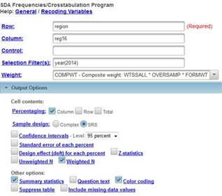
Let’s look at an example to help us better understand measures of association for nominal variables. We’re going to use two variables – region and reg16. The first variable – region – is the region of the country in which the respondent currently lives and the second – reg16 – is where the respondent lived at the age of 16. It would make sense to think of region as the dependent variable since where respondents lived at age 16 might influence where they currently live. Always put the dependent variable in the row and the independent variable in the column.[4]
Run CROSSTABS in SDA to produce the crosstabulation of region and reg16. Click on OUTPUT OPTIONS and look at PERCENTAGING. Since your independent variable is always in the column, you want to use the column percents. By default, the box for column percents is already checked. Also, click on OUTPUT OPTIONS and check the box for SUMMARY STATISTICS. Your screen should look like Figure 11-2. Notice that the SELECTION FILTER(S) box and the WEIGHT box are both filled in. Make sure that you selected SRS in the SAMPLE DESIGN line. Click on RUN THE TABLE to produce the crosstabulation.

Figure 11-2
Calculating C and V is easy. All you have to do is follow these simple steps.
- C equals the square root of the following: Chi Square divided by the sum of the number of cases in the table and Chi Square.
- Chi Square is the Pearson Chi Square. SDA expresses this as Chisq-P. (See Exercise STAT10S_SDA)
- Look at the SUMMARY STATISTICS that SDA gives you. The Pearson Chi Square is 10,268.34 and the number of cases in the table is 2,538.
- So divide 10,268.34 by the sum of 2,538 and 10,268.34. This equals 10,268.34 divided by 12,806.34 or 0.8018.
- Now take the square root of .8018 which equals 0.895.
- V equals the square root of the following: Chi Square divided by the product of the number of cases in the table and the smaller of two values – the number of rows minus 1 and the number of columns minus 1.
- The Pearson Chi Square is 10,268.34, the number of cases in the table is 2,538, the number of rows minus 1 is 9-1 or 8, the number of columns minus 1 is 10 – 1 or 9.
- The smaller of the number of rows minus 1 and the number of columns minus 1 is 8 since 9 -1 is smaller than 10 – 1.
- So divide 10,268.34 by the product of 2,538 and 8. This equals 10,268.34 divided by 20,304 or .5057.
- Now take the square root of .5057 which equals 0.711.
Notice that C and V are quite high. C is 0.895 and V is 0.711. You can see that C tells us that there is a very strong relationship between these two variables as does V.
Part V – Now it’s Your Turn
Use CROSSTABS in SDA to give you the table for race and region. The variable race classifies the respondents as white, black, or other. We want to find out whether the respondent’s race influences where the respondent currently lives. Decide which variable is independent and dependent. Remember to put the dependent variable in the row and the independent variable in the column. Get the correct percents and tell SDA to compute Chi Square. Then compute C and V by hand. Use all this information to describe the relationship between these two variables.
Part VI – Measures of Association for Ordinal Variables
There are a number of ordinal level variables in the 2014 GSS. Here are a few examples.
- respondent’s highest educational degree – degree
- spouse’s highest educational degree – spdeg
- satisfaction with current financial situation – satfin
- happiness with life – happy
- political views – polviews
You have a choice from four measures that SDA will compute for ordinal variables – Gamma, Somer’s d, Kendall’s tau-b, and Kendall’s tau-c. Let’s start with Somer’s d. This measure is the only one of the four that is an asymmetric measure. That means that Somer’s d allows you to specify one of the variables as independent and the other as dependent. Use CROSSTABS in SDA to get the crosstabulation of degree and satfin. If we think that education influences how satisfied respondents are with their financial situation, then satisfaction with financial situation would be our dependent variable and would go in the row and education would go in the column. Be sure to get the column percents, Chi Square, and the four measures of association we listed above.
Chi Square tells us that we should reject the null hypothesis that the two variables are unrelated which provides support for our research hypothesis that the variables are related to each other. Since satfin is our dependent variable the appropriate value of Somer’s d is
-.15. Tau-b and tau-c are very close to each other (-0.16 and -0.15). Gamma (-0.24) is larger. Gamma will always be larger because of the way it is computed.
Now let’s run a table using degree and spdeg. It doesn’t seem reasonable to treat one spouse’s education as independent and the other spouse’s education as dependent so let’s ignore Somer’s d.[5] In this example, it doesn’t matter which variable you put in the column and which you put in the row. Tab-b is 0.52 and tau-c is .46. Gamma as always is larger (0.69). The relationship between these two variables is clearly stronger than in the previous example.
You probably noticed that these measures for ordinal variables can be both positive and negative. The problem is that it’s hard to interpret the sign. We would like to be able to say that a positive value indicates that as one variable increases the other variable increases and a negative value indicates that as one variable increases the other variable decreases. But that depends on how the values are coded. So to determine whether a relationship is positive or negative it’s better to look at the percentages and let them tell you if it is positive or negative. In the first example, the sign of the measures was negative but the percentages tell us that the relationship is actually positive. As education increases, the percent that are happy with their life goes up.
Part VII – Now it’s Your Turn Again
Use CROSSTABS to give you a table for degree and happy. We want to find out if the respondent’s education helps us understand why some say they are happier than others. Decide which variable is independent and dependent. Get the correct percents and tell SDA to compute Chi Square and the four measures of association we discussed. Use all this information to describe the relationship between these two variables.
Part VIII – Using Measures of Association to Compare Tables
The primary use of measures of association is to compare the strength of a relationship in several tables. You want to make sure that you compare the same measure of association across tables. Compare Gamma values to Gamma values and V values to V values. Rerun one of the tables that you created in Parts 5 and 7 but this time hold sex constant. Do this by moving sex to the control box which is right below the COLUMN box in the crosstabs dialog box. Now compare the appropriate measure of association to determine if the relationship is stronger for males or females or whether it doesn’t vary much by sex. Remember not to make too much out of small differences in the measures.
[1] See exercise STAT1S_SDA for a discussion of levels of measurement. Nominal variables have no underlying order and ordinal variables have an underlying order. Measures of association for nominal variables range from 0 to 1 while measures for ordinal variables range from -1 to +1.
[2] There’s another popular measure called Lambda but SDA doesn’t compute it and it’s harder to compute by hand so we’re going to skip it.
[3] If your table has two columns and two rows, V is equal to Phi which you might be familiar with. Since Phi is a special case of V, we’re not going to discuss it.
[4] That’s important because as we noted earlier some measures are asymmetric which means that it depends on which of the two variables is dependent and which is independent. In these cases, SDA assumes that the row variable is the dependent variable.
[5] There is a symmetric value for Somer’s d which SDA does not compute.

