Author: Ed Nelson
Department of Sociology M/S SS97
California State University, Fresno
Fresno, CA 93740
Email: ednelson@csufresno.edu
Note to the Instructor: This exercise uses the 2014 General Social Survey (GSS) and SDA to explore crosstabulation. SDA (Survey Documentation and Analysis) is an online statistical package written by the Survey Methods Program at UC Berkeley and is available without cost wherever one has an internet connection. The 2014 Cumulative Data File (1972 to 2014) is also available without cost by clicking here. For this exercise we will only be using the 2014 General Social Survey. A weight variable is automatically applied to the data set so it better represents the population from which the sample was selected. You have permission to use this exercise and to revise it to fit your needs. Please send a copy of any revision to the author. Included with this exercise (as separate files) are more detailed notes to the instructors and the exercise itself. Please contact the author for additional information.
I’m attaching the following files.
- Extended notes for instructors (MS Word; .docx format).
- This page (MS Word; .docx format).
Goals of Exercise
The goal of this exercise is to introduce crosstabulation as a statistical tool to explore relationships between variables. The exercise also gives you practice in using CROSSTABS in SDA.
Part I—Relationships between Variables
In exercises STAT6S_SDA and STAT8S_SDA we used sample means to analyze relationships between variables. For example, we compared men and women to see if they differed in the number of years of school completed and the number of hours they worked in the previous week and discovered that men and women had about the same amount of education but that men worked more hours than women. We were able to compute means because years of school completed and hours worked are both ratio level variables (see STAT1S_SDA) The mean assumes interval or ratio level measurement (see STAT2S_SDA).
But what if we wanted to explore relationships between variables that weren’t interval or ratio? Crosstabulation can be used to look at the relationship between nominal and ordinal variables. Let’s compare men and women (sex) in terms of the following.
- opinion about abortion (abany)
- fear of crime (fear)
- satisfaction with current financial situation (satfin)
- opinion about gun control (gunlaw)
- gun ownership (owngun)
- voting (pres08),
- religiosity (reliten)
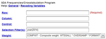
We’re going to use the General Social Survey (GSS) for this exercise. The GSS is a national probability sample of adults in the United States conducted by the National Opinion Research Center (NORC). The GSS started in 1972 and has been an annual or biannual survey ever since. For this exercise we’re going to use the 2014 GSS. To access the GSS cumulative data file in SDA format click here. The cumulative data file contains all the data from each GSS survey conducted from 1972 through 2014. We want to use only the data that was collected in 2014. To select out the 2014 data, enter year(2014) in the Selection Filter(s) box. Your screen should look like Figure 8-1. This tells SDA to select out the 2014 data from the cumulative file.

Figure 9-1
Notice that a weight variable has already been entered in the WEIGHT box. This will weight the data so the sample better represents the population from which the sample was selected.
The GSS is an example of a social survey. The investigators selected a sample from the population of all adults in the United States. This particular survey was conducted in 2014 and is a relatively large sample of approximately 2,500 adults. In a survey we ask respondents questions and use their answers as data for our analysis. The answers to these questions are used as measures of various concepts. In the language of survey research these measures are typically referred to as variables. Often we want to describe respondents in terms of social characteristics such as marital status, education, and age. These are all variables in the GSS.
Before we look at the relationship between sex and these other variables, we need to talk about independent and dependent variables. The dependent variable is whatever you are trying to explain. In our case, that would be how people feel about abortion, fear of crime, gun control and ownership, voting and religiosity. The independent variable is some variable that you think might help you explain why some people think abortion should be legal and others think it shouldn’t be legal or any of the other variables in our list above. In our case, that would be sex. Normally we put the dependent variable in the row and the independent variable in the column. We’ll follow that convention in this exercise.
Let’s start with the first two variables in our list. We’re going to use abany as our measure of opinion about abortion. Respondents were asked if they thought abortion ought to be legal for any reason. And we’re going to use fear as our measure of fear of crime. Respondents were asked if they were afraid to walk alone at night in their neighborhood. Run CROSSTABS in SDA to produce two tables. One will be for the relationship between sex and abany. The other will be for sex and fear. Put the independent variable in the column and the dependent variable in the row. SDA can compute the row percents, column percents, and total percents. Click on OUTPUT OPTIONS and look at PERCENTAGING. By default, the box for column percents is already checked. Your screen should look like Figure 9-2.
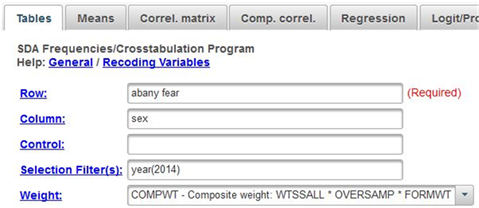
Figure 9-2
Your instructor will probably talk about how to compute these different percents. But how do you know which percents to ask for? Here’s a simple rule for computing percents.
- If your independent variable is in the column, then you want to use the column percents.
- If your independent variable is in the row, then you want to use the row percents.
Since you put the independent variable in the column, you want the column percents.
Part II – Interpreting the Percents
Your first table should look like this.
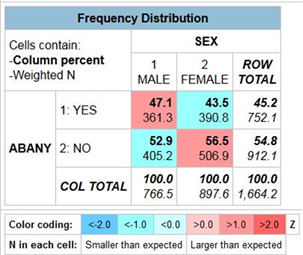
Figure 9-3
It’s easy to make sure that you have the correct percents. You independent variable (sex) should be in the column and it is. Column percents should sum down to 100% and they do.
How are you going to interpret these percents? Here’s a simple rule for interpreting percents.
- If your percents sum down to 100%, then compare the percents across.
- If your percents sum across to 100%, then compare the percents down.
Since the percents sum down to 100%, you want to compare across.
Look at the first row. Approximately 47% of men think abortion should be legal for any reason compared to 44% of women. There’s a difference of 3.6% which is really small. We never want to make too much of small differences. Why not? No sample is ever a perfect representation of the population from which the sample is drawn. This is because every sample contains some amount of sampling error. Sampling error in inevitable. There is always some amount of sampling error present in every sample. The larger the sample size, the less the sampling error and the smaller the sample size, the more the sampling error. So in this case we would conclude that there probably isn’t any difference in the population between men and women in their approval of abortion for any reason.
Now let’s look at your second table.

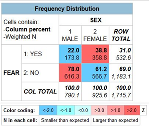
Figure 9-4
This time the percent difference is quite a bit larger. About 22% of men are afraid to walk alone at night in their neighborhood compared to 39% of women. This is a difference of 16.8%. This is a much larger difference and we have reason to think that women are more fearful of being a victim of crime than men.
Part III – Now it’s Your Turn
Choose two of the tables from the following list and compare men and women.
- satisfaction with current financial situation (satfin)
- opinion about gun control (gunlaw)
- gun ownership (owngun)
- religiosity (reliten)
Make sure that you put the independent variable in the column and the dependent variable in the row. Be sure to ask for the correct percents. What are values of the percents that you want to compare? What is the percent difference? Does it look to you that there is much of a difference between men and women in the variables you chose?
Part IV – Adding another Variable into the Analysis
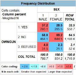
So far we have only looked at variables two at a time. Often we want to add other variables into the analysis. Let’s focus on the difference between men and women (sex) in terms of gun ownership (owngun). You might have run this table in Part III. If not, run the crosstab now. Here’s what you table should look like.

Figure 9-5
Notice that in this table “refused (3)” is in the rows. This is an example of missing data and we want to remove these cases from the table. We can do this by restricting the range for the variable owngun to the values 1 and 2. Enter the following into the row box – owngun(1-2). Now rerun the table and it ought to look like Figure 9-6.
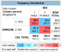
Figure 9-6
Men were more likely to own guns by 9.5%. But what if we wanted to include social class in this analysis? The 2014 GSS asked respondents whether they thought of themselves as lower, working, middle, or upper class. This is the variable class. What we want to do is to hold constant perceived social class. In other words, we want to divide our sample into four groups with each group consisting of one of these four classes and then look at the relationship between sex and owngun separately for each of these four groups.
We can do this by going back to the SDA dialog box where we requested the crosstabulation and putting the variable class in the CONTROL box right below the COLUMN box. Click on RUN THE TABLE to produce the results. Your tables should look like Figure 9-7.
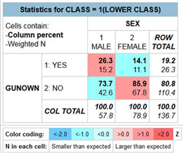
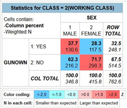
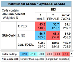
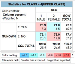
Figure 9-7
This table is more complicated. Notice that there are actually four tables. We often call them partial tables since each table contains part of the total sample. One of the tables is for those who said they were lower class, then working, middle and upper class. Let’s look at the percent differences for each of these tables – 12.2% (lower), 9.4% (working), 9.6% (middle), and 2.9% (upper). The first three tables are similar to the two-variable table – 9.5% compared to 12.2%, 9.4%, and 9.6%. The last table for upper class has a much smaller difference – 2.9%. We need to remember not to make too much out of small differences because of sampling error. In other words, when we look at only those who see themselves as upper class, there really isn’t much of a difference between men and women in terms of gun ownership.
But notice something else. There are fewer people who say they are lower and upper class than say they are working or middle class. There are only 137 respondents in the lower class table and even fewer, 48 respondents, in the upper class table. We’ll have more to say about this in the next exercise (STAT10S_SDA).
Part V – Now it’s Your Turn Again
In Part II we compared men and women (sex) in terms of fear of crime (fear). Run this table again but this time add social class (class) into the analysis as a control variable as we did in Part IV. What happens to the percent difference when you hold constant class? What does this tell you?

