Author: Ed Nelson
Department of Sociology M/S SS97
California State University, Fresno
Fresno, CA 93740
Email: ednelson@csufresno.edu
Note to the Instructor: This exercise uses the 2014 General Social Survey (GSS) and SDA to explore measures of skewness and kurtosis. SDA (Survey Documentation and Analysis) is an online statistical package written by the Survey Methods Program at UC Berkeley and is available without cost wherever one has an internet connection. The 2014 Cumulative Data File (1972 to 2014) is also available without cost by clicking here. For this exercise we will only be using the 2014 General Social Survey. A weight variable is automatically applied to the data set so it better represents the population from which the sample was selected. You have permission to use this exercise and to revise it to fit your needs. Please send a copy of any revision to the author. Included with this exercise (as separate files) are more detailed notes to the instructors and the exercise itself. Please contact the author for additional information.
I’m attaching the following files.
- Extended notes for instructors (MS Word; .docx format).
- This page (MS Word; .docx format).
Goals of Exercise
The goal of this exercise is to explore measures of skewness and kurtosis. The exercise also gives you practice in using FREQUENCIES in SDA.
Part I – Measures of Skewness
A normal distribution is a unimodal (i.e., single peak) distribution that is perfectly symmetrical. In a normal distribution the mean, median, and mode are all equal. Here’s a graph showing what a normal distribution looks like.
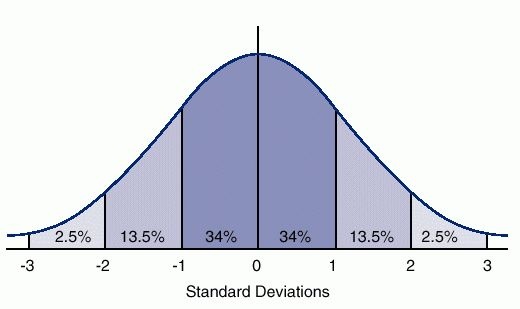
The horizontal axis is marked off in terms of standard scores where a standard score tells us how many standard deviations a value is from the mean of the normal distribution. So a standard score of +1 is one standard deviation above the mean and a standard score of -1 is one standard deviation below the mean. The percents tell us the percent of cases that you would expect between the mean and a particular standard score if the distribution was perfectly normal. You would expect to find approximately 34% of the cases between the mean and a standard score of +1 or -1. In a normal distribution, the mean, median, and mode are all equal and are at the center of the distribution. So the mean always has a standard score of zero.
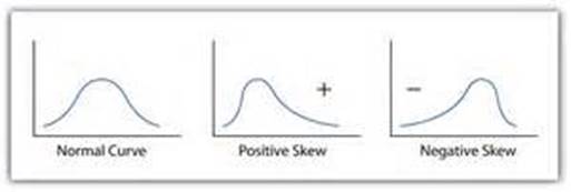
Skewness measures the deviation of a particular distribution from this symmetrical pattern. In a skewed distribution one side has longer or fatter tails than the other side. If the longer tail is to the left, then it is called a negatively skewed distribution. If the longer tail is to the right, then it is called a positively skewed distribution. One way to remember this is to recall that any value to the left of zero is negative and any value to the right of zero is positive. Here are graphs of positively and negatively skewed distributions compared to a normal distribution.
We’re going to use the General Social Survey (GSS) for this exercise. The GSS is a national probability sample of adults in the United States conducted by the National Opinion Research Center (NORC). The GSS started in 1972 and has been an annual or biannual survey ever since. For this exercise we’re going to use the 2014 GSS. To access the GSS cumulative data file in SDA format click here. The cumulative data file contains all the data from each GSS survey conducted from 1972 through 2014. We want to use only the data that was collected in 2014. To select out the 2014 data, enter year(2014) in the Selection Filter(s) box. Your screen should look like Figure 3-1. This tells SDA to select out the 2014 data from the cumulative file.
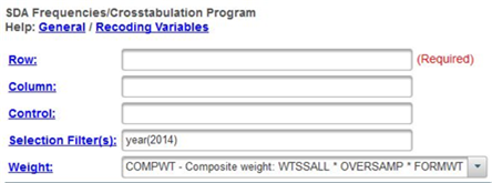
Figure 3-1
Notice that a weight variable has already been entered in the WEIGHT box. This will weight the data so the sample better represents the population from which the sample was selected.
The GSS is an example of a social survey. The investigators selected a sample from the population of all adults in the United States. This particular survey was conducted in 2014 and is a relatively large sample of approximately 2,500 adults. In a survey we ask respondents questions and use their answers as data for our analysis. The answers to these questions are used as measures of various concepts. In the language of survey research these measures are typically referred to as variables. Often we want to describe respondents in terms of social characteristics such as marital status, education, and age. These are all variables in the GSS.
Run FREQUENCIES in SDA for the variables age and sibs. To run the frequency distributions, enter the variable names, age and sibs, in the ROW box. Your screen should like Figure 3-2. Separate the variable names by either a space or a comma. Notice that the SELECTION FILTER(S) box and the WEIGHT box are both filled in.
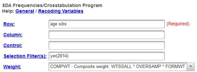
Figure 3-2
Once you have selected these variables click on the arrow next to OUTPUT OPTIONS and check the box for SUMMARY STATISTICS. Then click on CHART OPTIONS and click the arrow next to TYPE OF CHART. Select BAR CHART and now click on RUN THE TABLE at the bottom. SDA will compute the mean and median (plus other statistics) for each variable along with the bar chart.
Notice that the mean is larger than the median for both variables. This means that the distribution is positively skewed. But also notice that the mean for sibs is quite a bit larger than the median in a relative sense than is the case for age. This suggests that the distribution for sibs is the more skewed of the two variables. Look at the bar charts and you’ll see the same thing. Both variables are positively skewed but sibs is the more skewed variable. Now look at the skewness values — 1.72 for sibs and .24 for age. The larger the skewness value, the more skewed the distribution. Positive skewness values indicate a positive skew and negative values indicate a negative skew. There are various rules of thumb suggested for what constitutes a lot of skew but for our purposes we’ll just say that the larger the value, the more the skewness and the sign of the value indicates the direction of the skew.
Run FREQUENCIES for the following variables. Tell SDA to give you the bar chart along with the summary statistics. Write a paragraph for each variable explaining what these statistics tell you about the skewness of the variables.
- hrsrelax
- tvhours
Part II – Measures of Kurtosis
Kurtosis refers to the flatness or peakness of a distribution relative to that of a normal distribution. Distributions that are flatter than a normal distribution are called platykurtic and distributions that are more peaked are called leptokurtic.
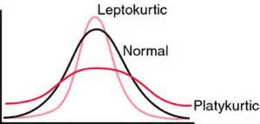
SDA will compute a kurtosis measure. Negative values indicate a platykurtic distribution and positive values indicate a leptokurtic distribution. The larger the kurtosis value, the more peaked or flat the distribution is.
Look back at the output for age and sibs. For age the kurtosis value was -.80 indicating a flatter distribution and for sibs kurtosis was 4.39 indicating a more peaked distribution. To see this visually look at your bar charts.
Run FREQUENCIES for the following variables. Tell SDA to give you the summary statistics and a bar chart. Write a paragraph for each variable explaining what these statistics tell you about the kurtosis of the variables.
- maeduc
- paeduc
- sexfreq


