Author: Ed Nelson
Department of Sociology M/S SS97
California State University, Fresno
Fresno, CA 93740
Email: ednelson@csufresno.edu
Note to the Instructor: This is the ninth in a series of 13 exercises that were written for an introductory research methods class. The first exercise focuses on the research design which is your plan of action that explains how you will try to answer your research questions. Exercises two through four focus on sampling, measurement, and data collection. The fifth exercise discusses hypotheses and hypothesis testing. The last eight exercises focus on data analysis. In these exercises we’re going to analyze data from one of the Monitoring the Future Surveys (i.e., the 2017 survey of high school seniors in the United States). This data set is part of the collection at the Inter-university Consortium for Political and Social Research at the University of Michigan. This data set is freely available to the public and you do not have to be a member of the Consortium to use it. We’re going to use SDA (Survey Documentation and Analysis) to analyze the data which is an online statistical package written by the Survey Methods Program at UC Berkeley and is available without cost wherever one has an internet connection. A weight variable is automatically applied to the data set so it better represents the population from which the sample was selected. You have permission to use this exercise and to revise it to fit your needs. Please send a copy of any revision to the author so I can see how people are using the exercises. Included with this exercise (as separate files) are more detailed notes to the instructors and the exercise itself. Please contact the author for additional information.
This page in MS Word (.docx) format is attached.
Goals of Exercise
The goal of this exercise is to introduce crosstabulation as a statistical tool to explore relationships between variables. The exercise also gives you practice in using CROSSTABS in SDA.
Part I—Relationships between Variables
We’re going to use the Monitoring the Future (MTF) Survey of high school seniors for this exercise. The MTF survey is a multistage cluster sample of all high school seniors in the United States. The survey of seniors started in 1975 and has been done annually ever since. To access the MTF 2017 survey follow the instructions in the Appendix. Your screen should look like Figure 9-1. Notice that a weight variable has already been entered in the WEIGHT box. This will weight the data so the sample better represents the population from which the sample was selected

Figure 9-1
MTF is an example of a social survey. The investigators selected a sample from the population of all high school seniors in the United States. This particular survey was conducted in 2017 and is a relatively large sample of a little more than 12,000 seniors. In a survey we ask respondents questions and use their answers as data for our analysis. The answers to these questions are used as measures of various concepts. In the language of survey research these measures are typically referred to as variables.
In exercises 6RM, 7RM, and 8RM we described variables one-at-a-time which is typically referred to as univariate (i.e., one variable) analysis. For example, we computed the percent of men and women in the sample.
But what if we wanted to explore the relationship between variables? What if we wanted to know if sex was related to binge drinking? (Binge drinking is often defined as having five or more drinks in a row.) Crosstabulation can be used to look at the relationship between nominal and ordinal variables (see exercise 6RM). When we look at the relationship between two variables, we often call this bivariate analysis.
Before we look at the relationship between two variables, we need to talk about independent and dependent variables. The dependent variable is whatever you are trying to explain. In our case, that would be why some students engage in binge drinking and others don’t. The independent variable is some variable that you think might help you explain why some students binge drink. In our case, that would be sex. Normally we put the dependent variable in the row and the independent variable in the column of our table. We’ll follow that convention in this exercise.
First, we have to locate the variable names for sex and binge drinking. On the left of the screen that you just opened you should see a mini-codebook. You can double click on any category in the codebook to see the list of variables in that category. Double click on “Demographic/Respondent Characteristics” and then on “Respondent Characteristics” and one of the variables should be the respondent's sex.
Now let's click on “Substance Use” and then on “Alcohol.” Now you can see that v2150 is the variable name for sex and that v2108 is the name for binge drinking. Since v2150 is the independent variable it should go in the column of our table and since v2108 is the dependent variable it will go in the row. Enter these variable names in the appropriate boxes.
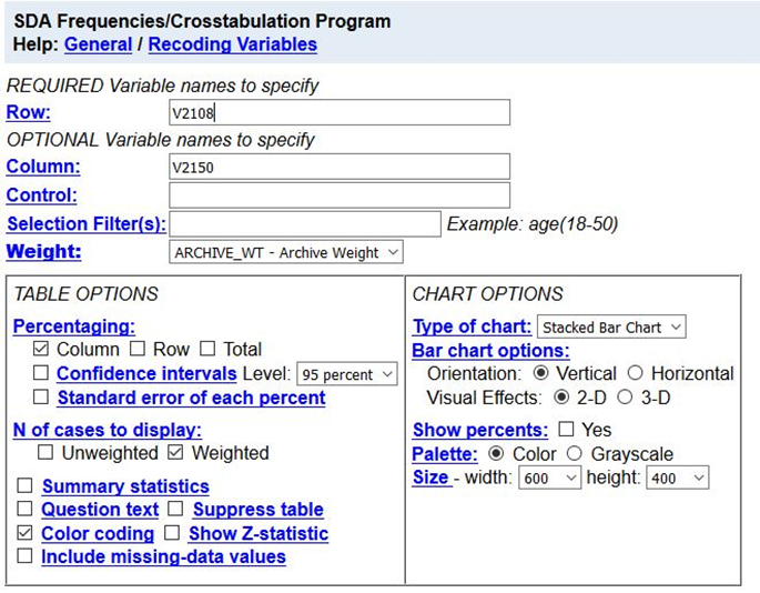
To interpret the table, you will need to compute percents. SDA can compute row percents, column percents, and total percents. Look at the “Table Options” section of your screen and you will see the boxes to check to indicate which percents you want SDA to compute. By default, the box for column percents is already checked. Your screen should look like Figure 9-2.

Figure 9-2
Your instructor will probably talk about how to compute these different percents. But how do you know which percents to ask for? Here’s a simple rule for computing percents.
- If your independent variable is in the column, then you want to use the column percents.
- If your independent variable is in the row, then you want to use the row percents.
Since you put the independent variable in the column, you want the column percents. Click on RUN THE TABLE to get the crosstabulation.
Part II – Interpreting the Percents
Your first table should look like this.
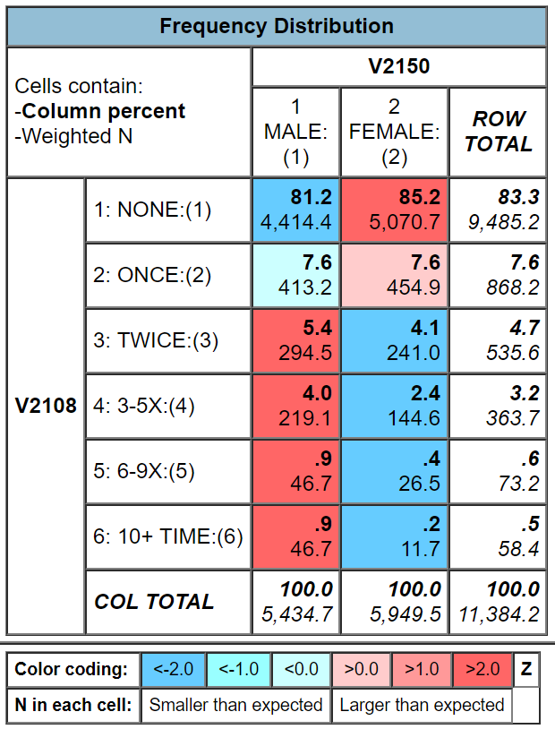
Figure 9-3
It’s easy to make sure that you have the correct percents. You independent variable (sex) should be in the column and it is. Column percents should sum down to 100% and they do.
How are you going to interpret these percents? Here’s a simple rule for interpreting percents.
- If your percents sum down to 100%, then compare the percents across.
- If your percents sum across to 100%, then compare the percents down.
Since the percents sum down to 100%, you want to compare across.
Look at the first row. Approximately 81% of men have never engaged in binge drinking compared to 85% of women. There’s a difference of 4% which is fairly small. We never want to make too much of small differences. Why not? No sample is ever a perfect representation of the population from which the sample is drawn. This is because every sample contains some amount of sampling error. Sampling error in inevitable. There is always some amount of sampling error present in every sample. The larger the sample size, the less the sampling error and the smaller the sample size, the more the sampling error. Since our sample size is so large, sampling error will be quite small. That means that in this case we can conclude that females are a little less likely to engage in binge drinking than men. If our sample size had been a lot smaller, we would have concluded there probably wasn’t much difference in the population between men and women for binge drinking. Note that we’re using our sample data to make inferences about the population.
Part III – Now it’s Your Turn
Choose two of the variables from the following list and compare men and women.
- how likely will attend a technical or vocational school after high school (v2180)
- how likely will graduate from a four-year college after high school (v2183)
- how likely will attend graduate or professional school after high school (v2184)
- how likely will serve in the armed services after high school (v2181)
Make sure that you put the independent variable in the column and the dependent variable in the row. Be sure to ask for the correct percents. What are values of the percents that you want to compare? What is the percent difference? Does it look to you that there is much of a difference between men and women in the population for the variables you chose? How did you decide?
So far, we have only looked at variables two at a time. Often, we want to add other variables into the analysis which is typically called multivariate analysis (i.e., analysis with more than two variables). We’ll consider multivariate analysis in exercise 12RM.

