RESEARCH METHODS 7RM - Central Tendency and Dispersion

Author:   Ed Nelson
Department of Sociology M/S SS97
California State University, Fresno
Fresno, CA 93740
Email:  ednelson@csufresno.edu

Note to the Instructor: This is the seventh in a series of 13 exercises that were written for an introductory research methods class.  The first exercise focuses on the research design which is your plan of action that explains how you will try to answer your research questions.  Exercises two through four focus on sampling, measurement, and data collection.  The fifth exercise discusses hypotheses and hypothesis testing.  The last eight exercises focus on data analysis.  In these exercises we’re going to analyze data from one of the Monitoring the Future Surveys (i.e., the 2017 survey of high school seniors in the United States).  This data set is part of the collection at the Inter-university Consortium for Political and Social Research at the University of Michigan.  This data set is freely available to the public and you do not have to be a member of the Consortium to use it.  We’re going to use SDA (Survey Documentation and Analysis) to analyze the data which is an online statistical package written by the Survey Methods Program at UC Berkeley and is available without cost wherever one has an internet connection.  A weight variable is automatically applied to the data set so it better represents the population from which the sample was selected.  You have permission to use this exercise and to revise it to fit your needs.  Please send a copy of any revision to the author so I can see how people are using the exercises. Included with this exercise (as separate files) are more detailed notes to the instructors and the exercise itself.  Please contact the author for additional information. 

This page in MS Word (.docx) format is attached.

Goal of Exercise

The goal of this exercise is to explore measures of central tendency (mode, median, and mean) and dispersion (range, standard deviation, and variance). The exercise also gives you practice in using FREQUENCIES in SDA.

Part I – Measures of Central Tendency

Data analysis always starts with describing variables one-at-a-time.  Sometimes this is referred to as univariate (one-variable) analysis.  Central tendency refers to the center of the distribution.

There are three commonly used measures of central tendency – the mode, median, and mean of a distribution.  The mode is the most common value or values in a distribution.[1]  The median is the middle value of a distribution.[2] The mean is the sum of all the values divided by the number of values.

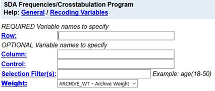
We’re going to use the Monitoring the Future (MTF) Survey of high school seniors for this exercise.  The MTF survey is a multistage cluster sample of all high school seniors in the United States.  The survey of seniors started in 1975 and has been an annual survey ever since. To access the MTF 2017 survey follow the instructions in the Appendix.   Your screen should look like Figure 7-1.  Notice that a weight variable has already been entered in the WEIGHT box.  This will weight the data so the sample better represents the population from which the sample was selected.

Figure 7-1

MTF is an example of a social survey.  The investigators selected a sample from the population of all high school seniors in the United States.  This particular survey was conducted in 2017 and is a relatively large sample of a little more than 12,000 students.  In a survey we ask respondents questions and use their answers as data for our analysis.  The answers to these questions are used as measures of various concepts.  In the language of survey research these measures are typically referred to as variables. 

Run FREQUENCIES in SDA for the variable v2196.  This variable is the number of miles per week that students drive.  Here’s the question from the survey – “During an average week, how much do you usually drive a car, truck, or motorcycle?”  To run the frequency distribution, enter the variable name, v2196, in the ROW box.  The WEIGHT box is already filled in.  Click on RUN THE TABLE to get the frequency distribution.  Your screen should look like Figure 7-2.

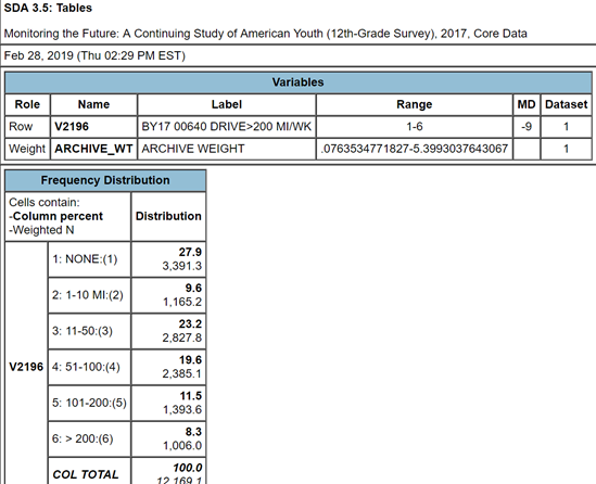
Figure 7-2

The responses to this question were divided into a set of six categories – none, 1 to 10, 11 to 50, 51 to 100, 101 to 200, and more than 200.  This was done to make the question easier to answer.  It’s difficult for respondents to remember the precise number of miles they drove per week.  It’s a lot easier to select one of these categories.  But this means that we don’t have the exact number of miles driven.  Keep that in mind as we think about measures of central tendency.

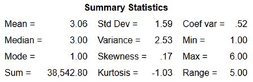
Rerun the table but this time check the box for SUMMARY STATISTICS under TABLE OPTIONS and click on the drop-down arrow next to TYPE OF CHART and select BAR CHART.  Below the frequency distribution you should see the statistics that SDA computes for you and the bar chart.  The summary statistics should look like Figure 7-3.

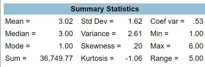
Figure 7-3

Your output will display a number of summary statistics.  Three of these statistics are commonly used measures of central tendency – mode, median, and mean.

• Mode = 1 meaning that the first category, none, was the most common answer (27.9%) from the 12,169 respondents who answered this question.  However, not far behind are those who drove 11 to 50 miles (23.2%).  So while technically the first category (none) is the mode, what you really found is that the most common values are one (none) and three (11 to 50 miles).  Another part of your output is the bar chart which is a chart or graph of the frequency distribution.  The bar chart clearly shows that categories one and three are the most common values (i.e., the highest bars in the bar chart) with category 4 not far behind.  So we would want to report that these two categories are the most common responses.
   
• Median = 3 which means that the third category, 11 to 50 miles, is the middle category for this distribution.  The middle category is the category that contains the 50^th percentile which is the value that divides the distribution into two equal parts.   In other words, it’s the value that has 50% of the cases above it and 50% of the cases below it.  If you added up the percents for all values less than 3 and the percents for all values less than or equal to  3, you would find that 37.5% of the cases drove 10 miles or less and that 60.7% of the cases drove 50 miles or less.  So the middle case (i.e., the 50^th percentile) falls somewhere in the category of 11 to 50 miles.  That is the median category.
   
• Mean = 3.02.  Clearly this is wrong.  The mean number of miles driven can’t be 3.02 miles.  SDA has computed the mean of the categorical values for this variable.  In other words, SDA has added up all the 1’s, 2’s, 3’s, 4’s, 5’s, and 6’s and divided that sum by the total number of cases.  Notice that SDA gives you the sum which is 36,749.77.  To get the mean, SDA divided that sum by 12,169.1 which equals 3.02 which is the mean of the categorical values.[3]  Let’s see if we can figure out a way to get SDA to compute the actual mean and not just the mean of the categorical values.

We can do this be changing the categorical values so they are the midpoint of the miles driven for each category.  That would mean we would have to do the following.

• We would change the categorical value of 1 to 0 which is the number of miles driven for this category.
• Change 2 to 5.5 which is the midpoint of category 2. To find the midpoint, add the smallest value in this category (1) and the largest value (10) and divide that sum by 2.
• Change 3 to 30.5 following the same procedure as above.
• Change 4 to 75.5.
• Change 5 to 150.5.
• Change 6 to 250.5.  Notice we have a problem here.  There is no upper limit to this category.  It’s simply more than 200.  We’re going to assume that nobody drives more than 300 miles per week and use 300 as our upper limit.  We have no way of knowing what the upper limit is so we’ll make what seems like a reasonable guess.

How are we going to tell SDA to make these changes?  By the way, this is called recoding.  We’re recoding the categorical values of 1, 2, 3, 4, 5, and 6 into the values above.  Follow these steps to recode in SDA.

• Enter the variable name in the row box.  The variable name in this example is v2196.  (Don’t enter the period.)
• After the variable name, enter (r: where r stands for recode.
• Enter the new value you want to assign to the first recode followed by the original value.  In our case we want to assign the new value 0 to the old value 1 so this would be 0=1.  (Don’t enter the period.)
• If you want to assign a label to each category, enter the label in double quotation marks. For example, our recode for the first category would look like this – v2196 (r:0=1”none”;.  (Don’t enter the period.)  We’re going to omit the labels in this exercise for simplicity sake.
• One problem is that SDA won’t allow you to recode using a fractional value so we’re going to drop the .5 in the midpoints.  That means that we will enter the midpoints as 0, 5, 30, 75, 150, and 250.  This will give us a slight underestimate of the mean but by a very small amount.   
• Separate the recodes by a semicolon.
• Repeat this process for each recode.  For example, for the second category it would look this – 5=2.  (Don’t enter the period.)
• After the last recode, end the statement with a right parenthesis.
• This is what our recode statement would look like – v2196(r:0=1;5=2;30=3;75=4;150=5;250=6).  (Don’t enter the period.)

Now tell SDA to compute the summary statistics for the recoded variable.  The mean should be 60.00 this time.  Notice that the mode is now 0 since that is the value for the first category and the median is 30 which is in the third category.  Remember that this is based on the assumption that all the cases in each category fall at the midpoint of that category.

Part II – Now it’s Your Turn

One of the variables in the data set is v2197 which is the number of driving tickets respondents received in the last twelve months.  The response categories are 0, 1, 2, 3, and 4 or more.  The only problem is the last open-ended category.  Let’s assume that no one received more than six tickets.  So the last category would be 4 to 6 with a midpoint of 5.  Follow the procedure described in Part I and compute the mode, median, and mean.  Write a paragraph discussing what these measures of central tendency mean.

Part III – Deciding Which Measure of Central Tendency to Use

The first thing to consider is the level of measurement (nominal, ordinal, interval, ratio) of your variable (see 6RM).

• If the variable is nominal, you have only one choice.  You must use the mode.
   
• If the variable is ordinal, you could use the mode or the median.  You should report both measures of central tendency since they tell you different things about the distribution.  The mode tells you the most common value or values while the median tells you where the middle of the distribution lies.
   
• If the variable is interval or ratio, you could use the mode or the median or the mean.  Now it gets a little more complicated.  There are several things to consider.
  • How skewed is your distribution?  Go back and look at the bar chart for v2196. Notice that there is a long tail to the right of the distribution.  The category with the largest number of cases is the first category which represents those who did not drive at all.  But there are quite a few respondents who report driving quite a bit.  For example, 11.5% report driving between 101 and 200 miles and 8.3% said they drive more than 200 miles per week.  That’s what we call a positively skewed distribution where there is a long tail towards the right or the positive direction. Now look at the median and mean for the recoded variable.  The mean (60.00) is larger than the median (30.0).  The respondents that drove a lot miles pull the mean up.  That’s what happens in a skewed distribution.  The mean is pulled in the direction of the skew.  The opposite would happen in a negatively skewed distribution.  The long tail would be towards the left and the mean would be lower than the median.  In a heavily skewed distribution the mean is distorted and pulled considerably in the direction of the skew.  So consider reporting only the median in a heavily skewed distribution.  That’s why you almost always see median income reported and not mean income.  Imagine what would happen if your sample happened to include Bill Gates.  The income distribution would have this very, very large value which would pull the mean up but not affect the median.
  • Is there more than one clearly defined peak in your distribution?   For example, consider a hypothetical distribution of 100 cases in which there are 50 cases with a value of two and fifty cases with a value of 8.  The median and mean would be five but there are really two centers of this distribution – two and eight.  The median and the mean aren’t telling the correct story about the center. You’re better off reporting the two clearly defined peaks of this distribution and not reporting the median and mean.

Run FREQUENCIES for the following variables.  Once you have entered the variable names in the ROW box, ask for the SUMMARY STATISTICS and a BAR CHART.  For each variable write a sentence or two indicating which measure(s) of central tendency (i.e., mode or median) would be appropriate to use to describe the center of the distribution and what the values of those statistics mean.  For some variables there will be more than one appropriate measure of central tendency.

• v49 – number of siblings
• v2108 – number of times had five drinks in a row in last two weeks
• v2116 – number of times used marijuana or hashish in last 12 months
• v2151 – race
• v2169 – how often attend religious services
• v2173 – how rate self on school ability

Part IV – Measures of Dispersion or Variation

Dispersion or variation refers to the degree that values in a distribution are spread out or dispersed.  The most commonly used measures – range, standard deviation, variance – are only appropriate for interval and ratio level variables (see exercise 6RM). The variables in the MTF survey are entirely nominal and ordinal variables but as you have seen in this exercise we can recode some of these variables so they are ratio variables.

The range is the difference between the highest and the lowest values in the distribution.  We don’t actually know the highest value for v2196 since the last category is more than 200 miles.  Earlier in this exercise we assumed that the largest value was 300.  If that is the case, what would the range be for the recoded variable? 

The range is not a very stable measure since it depends on the two most extreme values – the highest and lowest values.  These are the values most likely to change from sample to sample.

The variance is the sum of the squared deviations from the mean divided by the number of cases minus 1 and the standard deviation is just the square root of the variance.  Your instructor may want to go into more detail on how to calculate the variance by hand.  Look back at the summary statistics for your recode of v2196.  The variance equals 5,458.65.  What will the standard deviation equal?

The variance and the standard deviation can never be negative.  A value of 0 means that there is no variation or dispersion at all in the distribution.  All the values are the same.  The more variation there is, the larger the variance and standard deviation.

So what does the variance and the standard deviation for v2196 mean?  That’s hard to answer because you don’t have anything to compare it to.  But if you knew the standard deviation for both men and women you would be able to determine whether men or women have more variation.  Instead of comparing the standard deviations for men and women you would compute a statistic called the Coefficient of Relative Variation (CRV).  CRV is equal to the standard deviation divided by the mean of the distribution.   A CRV of 2 means that the standard deviation is twice the mean and a CRV of 0.5 means that the standard deviation is one-half of the mean.  You would compare the CRV’s for men and women to see whether men or women have more variation relative to their respective means.

How do we get SDA to compute the means and standard deviations for both men and women?  Click on ANALYSIS and then on COMPARISON OF MEANS in the blue horizontal bar at the top of your screen.  Enter the variable for which you want to compute the mean and standard deviation in the DEPENDENT box.  We're going to use the same variable we used in part I (v2196).  Be sure to enter the recode that you used in part 1.  Enter the variable (V2150) that you want to use to divide the sample into men and women in the ROW box.  SDA will automatically calculate the mean number of miles driven for both men and women.  To get the standard deviations, check the STD DEV box under TABLE OPTIONS.  Uncheck the STD ERRORS box under TABLE OPTIONS since you won’t need this statistic.  The mean will be the top number in each box of your output and the standard deviation will be right below the mean.  Compute the Coefficient of Variation for both men and women and write a sentence or two discussing whether men or women have more variation.

By the way, you might also have wondered why you need both the variance and the standard deviation when the standard deviation is just the square root of the variance.  You’ll just have to take my word for it that you will need both as you go further in statistics.